Equivalent Circuit Fitting
pypalmsens.fitting.CircuitModel fits the equivalent circuit specified with the CDC descriptor code. Optional settings are fixing the value of a parameter, setting the min/max bounds for a parameter, specifying the frequency range to fit, limiting the number of iterations, delta error term or delta parameter term.
Example usage for fitting an equivalent circuit:
>>> import pypalmsens as ps

>>> measurements = ps.load_session_file('examples/Demo CV DPV EIS IS-C electrode.pssession')
>>> eis_data = measurements[2].eis_data[0]

>>> cdc = 'R(RC)'
>>> model = ps.fitting.CircuitModel(cdc=cdc)
>>> result = model.fit(eis_data)
>>> result
FitResult(cdc='R(RC)', parameters=[134.2601648341703, 11839.397430811792, 4.763069310462662e-07], error=[...], ...)
result is an instance of pypalmsens.fitting.FitResult, a dataclass with fit values, errors, and other fitting data:
>>> result.cdc
'R(RC)'

>>> result.parameters
[134.2601648341703, 11839.397430811792, 4.763069310462662e-07]

>>> result.error
[2.3519772735560074, 2.466430045381699, 2.7610107312609493]

>>> result.n_iter
19

>>> result.chisq
0.014493966401698677

>>> result.exit_code
'MinimumDeltaErrorTerm'
CircuitModel takes a single parameter, the circuit description code (CDC).
Note that the code must be in all caps. For more information, see the CDC documentation.
You can pass result.parameters back to pypalmsens.fitting.CircuitModel.fit) to redo the fit from different starting parameters:
>>> model.fit(eis_data, parameters=result.parameters)
FitResult(cdc='R(RC)', parameters=[...], ...)
Parameters
If you want to tune the parameters, like fixing values or setting bounds, you can set them using the pypalmsens.fitting.Parameters class.
model.default_parameters grabs the default parameters for the CDC.
These can be modified, for example:
>>> parameters = model.default_parameters()

>>> parameters[0].value = 123  # set starting value to 123
>>> parameters[0].fixed = True # fix this value
>>> parameters[1].min = 12  # set lower bound
>>> parameters[1].max = 34  # set upper bound

>>> model.fit(eis_data, parameters=parameters)
FitResult(cdc='R(RC)', parameters=[...], error=[...], ...)
Re-fit EIS data
If you have already fitted your data in PSTrace, you can redo the fit or use the values as starting parameters:
>>> model = ps.fitting.CircuitModel(cdc=eis_data.cdc)
>>> model.fit(eis_data, parameters=eis_data.cdc_values)
FitResult(cdc='R([RT]Q)', parameters=[...], error=[...], ...)
Plotting
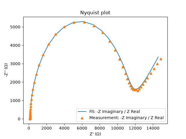
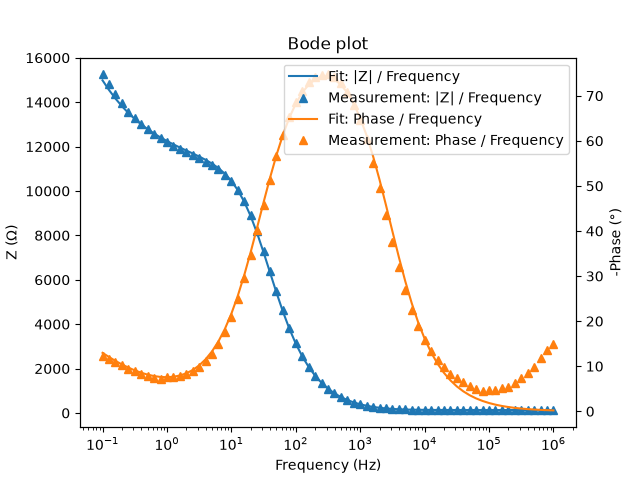
If you have matplotlib installed, you can generate the plots from the result:
>>> result.plot_nyquist(eis_data)
<Figure size 640x480 with 1 Axes>

>>> result.plot_bode(eis_data)
<Figure size 640x480 with 2 Axes>
Default values
This table shows the default values, the element types used in the system. Note that some element types have multiple values.
For more information on the formulas, please see the chapter "Equivalent Circuit Fitting" in the PSTrace user manual.
| Element | Value | Min | Max | Units |
|---|---|---|---|---|
| Resistance (R) | 1 × 10³ | 1 × 10⁻⁶ | 1 × 10¹² | Ω |
| Capacitance (C) | 10 × 10⁻⁹ | 1 × 10⁻¹² | 1 × 10⁻³ | F |
| Inductance (L) | 100 × 10⁻⁶ | 1 × 10⁻¹² | 1 × 10⁻³ | H |
| Constant Phase Element (Q) | ||||
| Y0 | 1 × 10⁻³ | 1 × 10⁻¹² | 1 × 10⁻³ | T |
| Constant phase exponent n | 1 | 0 | 1 | σ |
| Warburg (W) | 1 × 10³ | 1 × 10⁻⁶ | 1 × 10¹² | σ |
| Warburg Open (T) / Short (O) | ||||
| Warburg coefficient | 1 × 10³ | 1 × 10⁻⁶ | 1 × 10¹² | σ |
| B | 1 | 1 × 10⁻¹² | 1 × 10⁶ | √s |
| Experimental parameter | 0.5 | 0 | 1 | φ |
| Gerischer (G) | ||||
| Z0 | 1 × 10³ | 1 × 10⁻⁶ | 1 × 10¹² | Z₀ |
| k (reaction rate) | 1 | 1 × 10⁻¹² | 1 × 10⁶ | s⁻¹ |
| Bisquert Open (M) / Short (N) | ||||
| Z pore | 100 | 1 × 10⁻⁶ | 1 × 10¹² | Ω |
| Reaction resistance | 10 × 10³ | 1 × 10⁻⁶ | 1 × 10¹² | Ω |
| Pore diffusion CPE T | 1 × 10⁻³ | 1 × 10⁻¹² | 1 × 10⁻³ | T |
| Pore diffusion CPE n | 1 | 0 | 1 | Φ |
| Pore depth | 1 | 0 | 1 × 10¹² | L |
Impedance.py
impedance.py is a popular Python package for analyzingelectrochemical impedance spectroscopy (EIS) data.
It has a a straightforward, scikit-learn-like API for impedance analysis.
You can install impedance.py via pip install impedance.
For more information, see the documentation or source code on Github.
From an eis data set, it is trivial to create the frequency and impedance data (Z) for impedance.py using numpy:
import pypalmsens as ps
import numpy as np

measurement = ps.load_session_file('examples/Demo CV DPV EIS IS-C electrode.pssession')[2]

eis = measurement.eis_data[0]

F = np.array(eis.dataset['Frequency'])
Zre = np.array(eis.dataset['ZRe'])
Zim = np.array(eis.dataset['ZIm'])

Z = Zre - 1j * Zim
For example, to fit this circuit model:
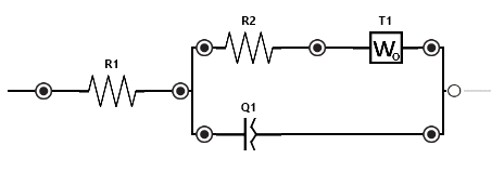
We can use the circuit description: 'R0-p(R1-Wo1,CPE1)'. This is different from the CDC codes used by PalmSens. You can read about the available elements here.
The example below shows how to fit the circuit model to the data:
import matplotlib.pyplot as plt
from impedance.models.circuits import CustomCircuit
from impedance.visualization import plot_nyquist

circuit = 'R0-p(R1-Wo1,CPE1)'

initial_guess = [1000, 1000, 1000, 0.5, 1e-6, 1]

circuit = CustomCircuit(circuit, initial_guess=initial_guess)

ret = circuit.fit(F, Z)

print(ret)

Z_fit = circuit.predict(F)

fig, ax = plt.subplots()
plot_nyquist(Z, fmt='o', scale=10, ax=ax)
plot_nyquist(Z_fit, fmt='-', scale=10, ax=ax)

plt.legend(['Data', 'Fit'])
plt.show()
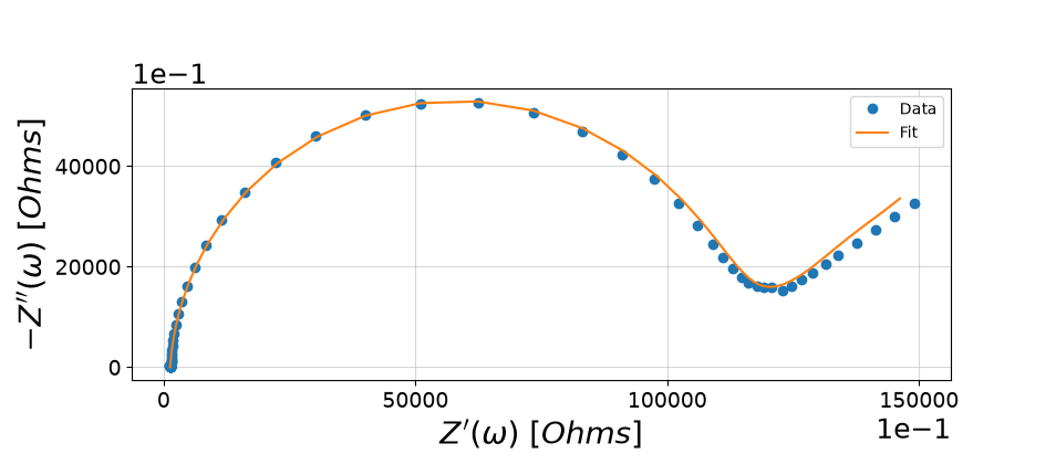
This results in the nyquist plot below: