Working with Data

This page shows how to use pypalmsens to interface with your measurement data.

The pypalmsens.data submodule contains wrappers for the data structure in the underlying PalmSens .NET SDK libraries.

Measurement

The top level object is a Measurement. The Measurement class contains information about the method, data, and experiment metadata.

>>> import pypalmsens as ps
>>> measurements = ps.load_session_file('examples/Demo CV DPV EIS IS-C electrode.pssession')
>>> measurements
[Measurement(title=Differential Pulse Voltammetry, timestamp=2017-07-12T14:28:58, device=PalmSens4), Measurement(title=Cyclic Voltammetry [1], timestamp=2017-07-12T14:33:10, device=PalmSens4), Measurement(title=Impedance Spectroscopy [2], timestamp=2017-07-12T14:48:42, device=PalmSens4)]

Note that a session file (.pssession) can contain multiple measurements. Therefore, pypalmsens.load_session_file always returns a list of measurements. You can select the first measurement (DPV) using index [0]:

>>> measurement = measurements[0]

Loading a single measurement

If you know your session file only contains a single measurement, you can use the convenience functions: pypalmsens.load_measurement and omit the index: measurement = ps.load_measurement('my_measurement.pssession')

From there, you can query device information and other metadata:

>>> measurement.device
DeviceInfo(type='PalmSens4', firmware='', serial='PS4A16A000003', id=9)

And measurement details like title and timestamp:

>>> measurement.title
'Differential Pulse Voltammetry'

>>> measurement.timestamp
'2017-07-12T14:28:58'

>>> measurement.channel # (1)!
-1

For multichannel measurements

You have two main ways to access the data:

measurement.dataset returns the raw data that were measured, analogous to the Data tab in PSTrace.
measurement.curves returns a list of Curve objects, which represent the plots.

For more information, see the pypalmsens.data.Measurement.

Curve

A measurement can contain multiple curves, therefore measurement.curves returns a list. The example below has only one curve with 219 data points:

>>> curves = measurement.curves
>>> curves
[Curve(title=Curve, n_points=219)]

>>> curve = curves[0]

You can query some Curve metadata like this:

>>> curve.title
'Curve'

>>> len(curve)
219

>>> curve.x_label, curve.x_unit
('Potential', 'V')

>>> curve.y_label, curve.y_unit
('Current', 'µA')

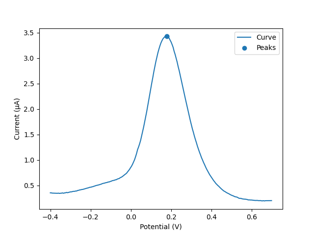
Use the .plot() method to visualize the data. This requires matplotlib to be installed:

>>> fig = curve.plot() # (1)!
>>> fig
<Figure size 640x480 with 1 Axes>

This returns a matplotlib.figure.Figure, use fig.show() to show the plot.

The resulting plot looks like this:

Image of DPV plot

Peak-finding

The measurement above stores a single peak. You can retrieve it using:

>>> peaks = curve.peaks
>>> peaks
[Peak(x=0.179102 V, y=3.42442 µA, y_offset=0.501758 µA, area=0.647762 VµA, width=0.201485 V)]

To programmatically find peaks, use .find_peaks():

>>> peaks = curve.find_peaks()
>>> peaks
[Peak(x=0.179102 V, y=3.42442 µA, y_offset=0.26371 µA, area=0.818265 VµA, width=0.216563 V)]

Alternatively, for Cyclic Voltammetry (CV) and Linear Sweep Voltammetry (LSV), you can use curve.find_peaks_semiderivative(). For more information on this algorithm, see this Wikipedia page.

Peak finding

The peak finder may not always find peaks on the first attempt depending on your data. You may need to tune parameters for better results. See pypalmsens.data.Curve.find_peaks for more information.

Smoothing

You can also filter data using pypalmsens.data.Curve.smooth. Note that this method updates the curve in-place:

>>> curve.smooth(smooth_level=1)

Or, you can use a Savitsky-Golay filter:

>>> curve.savitsky_golay(window_size=3)

Baseline correction

You can perform baseline correction using pypalmsens.data.Curve.remove_baseline.

This applies a moving-average baseline correction and returns the corrected curve and the calculated baseline. This function is equivalent to the 'Moving Average Baseline' function in PSTrace.

The function returns a BaselineResult named tuple, so you can unpack the two values directly:

>>> corrected, baseline = curve.remove_baseline(max_sweeps=500, window_size=2)

>>> corrected
Curve(title=Curve (corrected), n_points=219)

>>> baseline
Curve(title=Curve (baseline), n_points=219)

Or access them by name:

>>> result = curve.remove_baseline(max_sweeps=500, window_size=2)

>>> result.corrected
Curve(title=Curve (corrected), n_points=219)

>>> result.baseline
Curve(title=Curve (baseline), n_points=219)

Data access

Curve data are derived from the underlying Dataset, where variable data are stored in DataArray's. To access the raw x and y data for custom plotting or analysis, use curve.x_array and curve.y_array. Both return DataArray objects that can be converted to standard Python floats or numpy arrays:

>>> curve.x_array
DataArray(name=potential, unit=V, n_points=219)

>>> list(curve.x_array)
[-0.399962, -0.394962, ..., 0.692698, 0.697776]

>>> curve.y_array
DataArray(name=current, unit=µA, n_points=219)

>>> import numpy as np
>>> np.array(curve.y_array)
array([0.352146  , 0.34988091, ..., 0.19905777, 0.199557  ])

For more details on array manipulation, see pypalmsens.data.Curve.

Peak

Peak is a small dataclass containing peak properties. Stored peaks can be retrieved from a Curve (for example, if PSTrace stored peaks in the .pssession file):

>>> peaks = curve.peaks
>>> peaks
[Peak(x=0.179102 V, y=3.42408 µA, ...), Peak(x=0.179102 V, y=3.42408 µA, ...]

Many peak properties are accessible from this object:

>>> peak = peaks[0]
>>> peak.x, peak.y
(0.179102, 3.4240794)

>>> peak.width
0.2014852

>>> peak.area
0.64776224

>>> peak.left_x, peak.right_x
(-0.0626174, 0.481213)

>>> peak.value # (1)!
2.9223213

The peak.value represents the height of the peak relative to the baseline.

For more information on peak properties, see pypalmsens.data.Peak.

DataSet

Raw data are stored in a DataSet. The dataset contains all raw measurement data, including the data for the curves.

>>> dataset = measurement.dataset
>>> dataset
DataSet(['Time', 'Potential', 'Current'])

Since a DataSet acts like a Python dictionary (a mapping), you can access arrays by name:

>>> dataset['Time']
DataArray(name=time, unit=s, n_points=219)

>>> dataset['Potential']
PotentialArray(name=potential, unit=V, n_points=219)

To list all available arrays:

>>> dataset.arrays()
[DataArray(name=time, unit=s, n_points=219), PotentialArray(name=potential, unit=V, n_points=219), CurrentArray(name=current, unit=µA, n_points=219)]

You can retrieve arrays of a specific type using:

>>> sorted(dataset.array_types)  #(1)!
['Current', 'Potential', 'Time']

>>> dataset.arrays(type='Current')
[CurrentArray(name=current, unit=µA, n_points=219)]

dataset.array_types returns a set

Alternatively, you can query by name:

>>> sorted(dataset.array_names)
['current', 'potential', 'time']

>>> dataset.arrays(name='time')
[DataArray(name=time, unit=s, n_points=219)]

You can also filter by quantity:

>>> sorted(dataset.array_quantities)
['Current', 'Potential', 'Time']

>>> dataset.arrays(quantity='Potential')
[PotentialArray(name=potential, unit=V, n_points=219)]

Type and quantity may seem similar, but for methods with many quantities the difference will be visible. For example, in impedimetric measurements (EIS/GEIS), 'miDC' and 'Iac' are different array types, but have the same quantity: 'Current'.

Note that for larger datasets, these methods might return multiple DataArray objects. Data from a Cyclic Voltammetry measurement can contain multiple scans, meaning the dataset might hold multiple arrays per array type.

If you have pandas installed, you can easily convert the entire dataset into a DataFrame:

>>> import pandas as pd
>>> df = pd.DataFrame(dataset.to_dict())
>>> df
     Time  Potential   Current    CR ReadingStatus
0     0.0  -0.399962  0.352146  10uA            OK
1     0.2  -0.394962  0.351192  10uA            OK
2     0.4  -0.389884  0.346900  10uA            OK
...
216  43.2   0.687698  0.198544  10uA            OK
217  43.4   0.692698  0.199080  10uA            OK
218  43.6   0.697776  0.199557  10uA            OK
<BLANKLINE>
[219 rows x 5 columns]

Any new Curve can be generated by passing the desired x and y keys:

>>> list(dataset)
['Time', 'Potential', 'Current']

>>> curve = dataset.curve(x='Time', y='Potential', title='My curve')
>>> curve
Curve(title=My curve, n_points=219)

For more information on Dataset, see pypalmsens.data.DataSet.

DataArray

Data arrays store a list of values, essentially representing a single column in the PSTrace Data tab. A Dataset contains multiple data arrays.

Let's examine the first current array:

>>> array, *_ = dataset.arrays(type='Current')
>>> array
CurrentArray(name=current, unit=µA, n_points=219)

An array stores metadata about itself:

>>> array.name
'current'

>>> array.type
'Current'

>>> array.unit
'µA'

>>> array.quantity
'Current'

Arrays behave like a Python Sequence (e.g., a list):

>>> len(array)
219

>>> min(array)
0.193358

>>> max(array)
3.42442

>>> array[0]
0.352146

Arrays support complex slicing, but remember that this operation returns a standard Python list:

>>> array[:5]
[0.352146, 0.351192, 0.3469, 0.345947, 0.344516]

>>> array[-5:]
[0.197411, 0.198127, 0.198544, 0.19908, 0.199557]

>>> array[::-1]  # (1)!
[0.199557, 0.19908, ..., 0.351192, 0.352146]

reverse list

You can convert arrays into lists or numpy arrays:

>>> list(array)
[0.352146, 0.351192, ..., 0.19908, 0.199557]

>>> np.array(array)
array([0.352146, 0.351192, ..., 0.19908 , 0.199557])

For more information on array structures, see pypalmsens.data.DataArray.

CurrentArray

CurrentArray derives from DataArray and includes additional methods for analyzing current readings, such as the current range, reading status, etc.:

>>> array = dataset['Current']
>>> array
CurrentArray(name=current, unit=µA, n_points=219)

>>> array.current()  # (1)!
[0.352146, 0.351192, ..., 0.19908, 0.199557]

>>> array.current_in_range()  # (2)!
[0.0352146, 0.0351192, ..., 0.019908000000000002, 0.0199557]

>>> array.current_range()  # (3)!
['10uA', '10uA', ..., '10uA', '10uA']

>>> array.reading_status()  # (4)!
['OK', 'OK', ..., 'OK', 'OK']

>>> array.timing_status()  # (5)!
['Unknown', 'Unknown', ..., 'Unknown', 'Unknown']

>>> pd.DataFrame(array.to_dict())
      Current  CurrentInRange    CR TimingStatus ReadingStatus
0    0.352146        0.035215  10uA      Unknown            OK
1    0.351192        0.035119  10uA      Unknown            OK
2    0.346900        0.034690  10uA      Unknown            OK
...
216  0.198544        0.019854  10uA      Unknown            OK
217  0.199080        0.019908  10uA      Unknown            OK
218  0.199557        0.019956  10uA      Unknown            OK
<BLANKLINE>
[219 rows x 5 columns]

returns current readings in µA
returns values within a specified range
returns the current range bins (e.g., '100uA', '1mA')
returns status for each reading
returns timing status

For more information, see pypalmsens.data.CurrentArray.

PotentialArray

Similar to currents, PotentialArray also derives from DataArray and provides methods to query associated data:

>>> array = measurement.dataset['Potential']
>>> array.potential()  # (1)!
[-0.399962, -0.394962, ..., 0.692698, 0.697776]

>>> array.potential_in_range()  # (2)!
[-0.399962, -0.394962, ..., 0.692698, 0.697776]

>>> array.potential_range()  # (3)!
['1V', '1V', '1V', ...]

>>> array.reading_status()  # (4)!
['OK', 'OK', ..., 'OK', 'OK']

>>> array.timing_status()  # (5)!
['Unknown', 'Unknown', ..., 'Unknown', 'Unknown']

>>> pd.DataFrame(array.to_dict())
     Potential  PotentialInRange  CR TimingStatus ReadingStatus
0    -0.399962         -0.399962  1V      Unknown            OK
1    -0.394962         -0.394962  1V      Unknown            OK
2    -0.389884         -0.389884  1V      Unknown            OK
...
216   0.687698          0.687698  1V      Unknown            OK
217   0.692698          0.692698  1V      Unknown            OK
218   0.697776          0.697776  1V      Unknown            OK
<BLANKLINE>
[219 rows x 5 columns]

returns potential readings in V
returns values within a specified range
returns potential range bins (e.g., '1V')
returns status for each reading
returns timing status

For more information, see pypalmsens.data.PotentialArray.

EISData

You can retrieve impedance data from an impedance (EIS/GEIS) measurement.

Since an EIS measurement might be multichannel, .eis_data returns a list of results. If you are not using a multiplexer, you can select the first (and only) item from this list:

>>> eis_measurement = measurements[2]
>>> eis_measurement
Measurement(title=Impedance Spectroscopy [2], timestamp=2017-07-12T14:48:42, device=PalmSens4)

>>> eis_measurement.eis_data  # (1)!
[EISData(title=FixedPotential at 71 freqs [2], n_points=71, n_frequencies=71)]

>>> eis_data = eis_measurement.eis_data[0] # (2)!

.eis_data returns a list
pick the first and only item

The EISData object can be queried for metadata:

>>> eis_data.title
'FixedPotential at 71 freqs [2]'

>>> eis_data.scan_type
'fixed'

>>> eis_data.frequency_type
'scan'

>>> eis_data.n_points
71

>>> eis_data.n_frequencies
71

If you previously fitted a circuit model in PSTrace, you can retrieve the CDC values:

>>> eis_data.cdc
'R([RT]Q)'

>>> eis_data.cdc_values
[132.146, 11009.9, 3710.55, 3.77887, 0.971414, 6.23791e-07, 0.961612]

You can use these values to fit a circuit model:

>>> model = ps.fitting.CircuitModel(cdc=eis_data.cdc)
>>> result = model.fit(eis_data, parameters=eis_data.cdc_values)
>>> result
FitResult(cdc='R([RT]Q)', parameters=[...], error=[...], chisq=..., n_iter=5, exit_code='MinimumDeltaErrorTerm')

The raw data can be accessed via .dataset, which returns a DataSet object:

>>> eis_data.dataset
DataSet(['Current', 'Potential', 'Time', 'Frequency', 'ZRe', 'ZIm', 'Z', 'Phase', ...])

You can retrieve all arrays from the EIS data:

>>> eis_data.arrays()
[CurrentArray(name=Idc, unit=µA, n_points=71),
 PotentialArray(name=potential, unit=V, n_points=71),
 DataArray(name=time, unit=s, n_points=71),
 ...
 DataArray(name=Capacitance, unit=F, n_points=71),
 DataArray(name=Capacitance', unit=F, n_points=71),
 DataArray(name=Capacitance'', unit=F, n_points=71)]

For more information on EIS datasets, see pypalmsens.data.EISData.

Subscans

If an EIS dataset contains subscans, this will be shown in the object's representation:

>>> measurement = ps.load_measurement('tests/test_data/eis_3ch_4scan_5freq.pssession')
>>> measurement
Measurement(title=Impedance Spectroscopy, timestamp=2025-07-31T15:54:28, device=EmStat4HR)

>>> eis_data = measurement.eis_data[0]
>>> eis_data
EISData(title=CH 3: E dc scan at 5 freqs, n_points=20, n_frequencies=5, n_subscans=4)

>>> eis_data.has_subscans
True

>>> eis_data.n_subscans
4

Subscans can be accessed via the .subscans() method:

>>> eis_data.subscans
[EISData(title=E=0.000 V, n_points=5, n_frequencies=5),
 EISData(title=E=0.200 V, n_points=5, n_frequencies=5),
 EISData(title=E=0.400 V, n_points=5, n_frequencies=5),
 EISData(title=E=0.600 V, n_points=5, n_frequencies=5)]

Subscans are themselves EISData objects.